causal-inference-on-time-series-with-causal-impact

Notes: CausalImpact

Notes related to Causal Inference with CausalImpact, R Package from Google.

Why Causal Inference?

Let’s say we made changes to a policy, tool, campaign, or process we are running. We may want to answer the question of what effect did change X have on our service? The gold standard for estimating this effect is a randomized control trial. However, that might be too difficult, too expensive, unethical, or simply because it wasn’t done. Causal inference is a technique designed to help estimate the impact of a change in cases where a randomized experiment is not an option.

A simple example

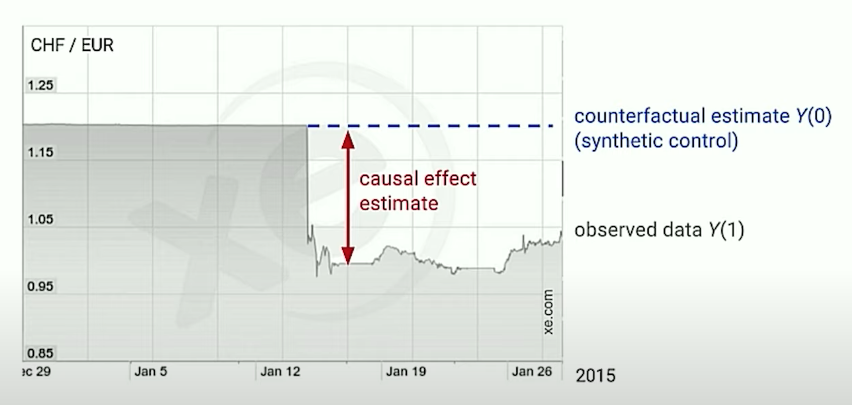
On January 15, 2015, the Swiss National Bank (SNB) announced it would no longer hold the Swiss franc at a fixed exchange rate with the euro. The image below shows the exchange rate before the announcement, the observed value after treatment (Y(1)) and the expected exchange rate if no announcement had been made (i.e., the counterfactual example Y(0)).

Swiss Franc to Euro Source: Youtube - Inferring the effect of an event using CausalImpact by Kay Brodersen

Key concepts in this image are:

Y(1) is our observed data, what actually happened after the treatment
Y(0) is our counterfactual estimate, or synthetic control, or the expected outcome with no treatment
the causal effect estimate is the difference between the observed Y(1) and the synthetic control Y(O), or the difference between the two outcomes.

The problem of causal inference

We cannot observe the potential outcomes with and without the treatment at the same time. For instance, we cannot see a single patient’s outcome if we administered and did not administer a drug at the same time. The outcomes are mutually exclusive; to address this, our options are.

Run a controlled experiment, where we see some of the potential outcomes with and without treatment.
Use observational methods, to try to estimate the effect in the absence of a controlled experiment.
Master time travel.

CausalImpact

What is the CausalImpact approach to this problem?

Building A Model

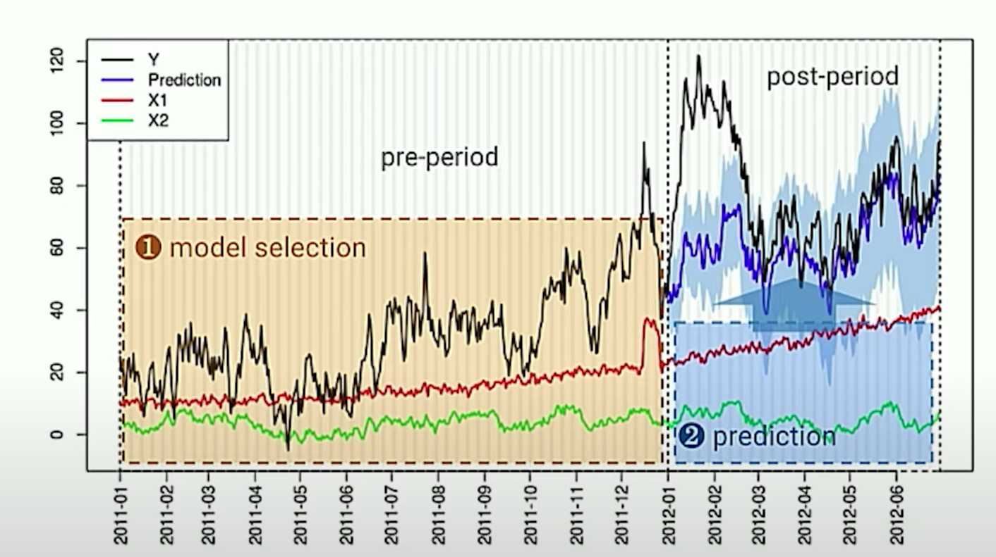
In order to use the CausalImpact package, we need a few things.

A time series of our target observation (Y)
- This time series must designate a pre-period and a post-period group.
One more co-variate, “predictor” time-series sets (X1, and X2), that they themselves are not impacted by the treatment at the time (t).
In a Bayesian Framework, any priors we want include (i.e., from previous studies)

We leverage these co-variate sets to estimate the synthetic-control, which we use to estimate our causal effect in the post-period.

A more complex
example Source: Youtube - Inferring the effect of an event using CausalImpact by Kay Brodersen

Assumptions

It is assumed we have:

One or more control (predictor) time series that they themselves are not affected by the intervention
The relationship between the covariates and the treated time series are established during the pre-period, and remain stable in the post period.

A Code

suppressMessages(library(zoo))
suppressMessages(library(CausalImpact))

# <https://google.github.io/CausalImpact/CausalImpact.html>
set.seed(1)
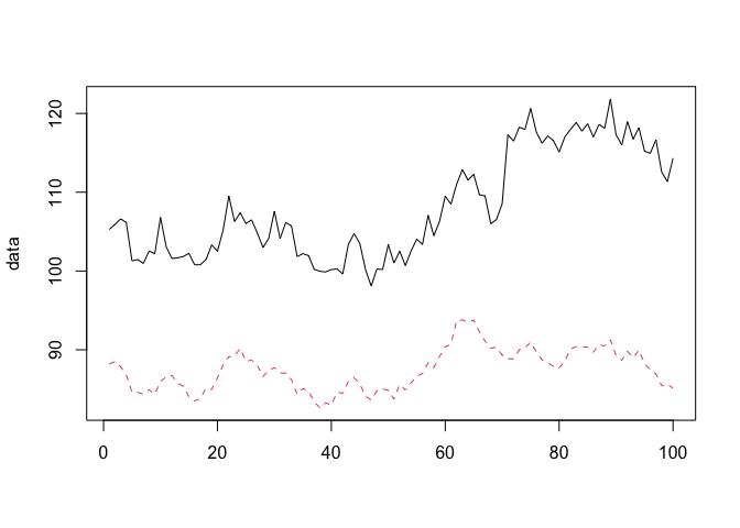
x1 <- 100 + arima.sim(model = list(ar = 0.999), n = 100) # generate covariate series
y  <- 1.2 * (x1) + rnorm(100)     
y[71:100] <- y[71:100] + 10
time.points <- seq.Date(as.Date("2014-01-01"), by = 1, length.out = 100)
data <- zoo(cbind(y, x1), time.points)
head(data)

##                   y       x1
## 2014-01-01 105.2950 88.21513
## 2014-01-02 105.8943 88.48415
## 2014-01-03 106.6209 87.87684
## 2014-01-04 106.1572 86.77954
## 2014-01-05 101.2812 84.62243
## 2014-01-06 101.4484 84.60650

matplot(data, type = "l")

pre.period <- as.Date(c("2014-01-01", "2014-03-11"))   # We need to tell the model what observations occurred prior to treatment
post.period <- as.Date(c("2014-03-12", "2014-04-10"))  # We also need to identify the post-treatment period

impact <- CausalImpact(data, pre.period, post.period)
plot(impact)

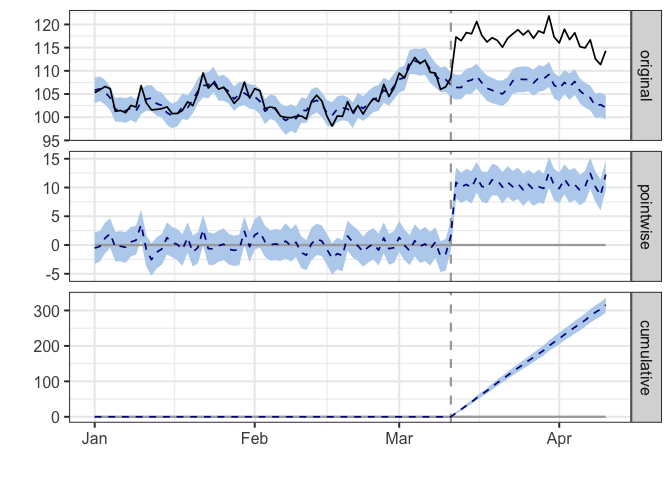
summary(impact)

## Posterior inference {CausalImpact}
## 
##                          Average        Cumulative  
## Actual                   117            3511        
## Prediction (s.d.)        107 (0.35)     3196 (10.38)
## 95% CI                   [106, 107]     [3176, 3217]
##                                                     
## Absolute effect (s.d.)   11 (0.35)      316 (10.38) 
## 95% CI                   [9.8, 11]      [294.4, 336]
##                                                     
## Relative effect (s.d.)   9.9% (0.32%)   9.9% (0.32%)
## 95% CI                   [9.2%, 11%]    [9.2%, 11%] 
## 
## Posterior tail-area probability p:   0.00101
## Posterior prob. of a causal effect:  99.8994%
## 
## For more details, type: summary(impact, "report")

Key Questions

Question: How many co-variate (predictor) time series do you need to successfully to this analysis?

Relying on a single co-variate time series runs the risk of reacting quickly to the specifics of the co-variate series. Instead, it is recommended that a handful or a few dozen co-variate time series be used. Enough to guard against spurious correlations, but few that you can understand and explain what each of these time series means.

Source: Youtube - Inferring the effect of an event using CausalImpact by Kay Brodersen @ 26:41

Question: Can you use this method to calculate the impact of multiple events if they overlap in time?

As of 2016, this was an open research question. Need to do additional research to determine if this is still true.

Source: Youtube - Inferring the effect of an event using CausalImpact by Kay Brodersen @ 28:21

Question: The causal impact estimate seems to be at the mercy of the credible intervals. Are tools to analyze and potentially reduce the confidence interval in that post-treatment period?

The confidence interval reflects the uncertainty in our prediction. As you get further out into the future, you are less certain of the output and expect that confidence interval to expand. The better your predictor series are explaining the target, the tighter your confidence intervals are likely to be. The inverse of that, if you don’t have any good predictor time series, then your confidence interval will be wide and reflect that uncertainty.

Source: Youtube - Inferring the effect of an event using CausalImpact by Kay Brodersen @ 28:42

Question: How do we identify ‘good’, covariate predictor time-series?

We want to find time series that are related to our outcome variable, to our original time series, but are not affected by out treatment. Consider a scenario when we launch an advertising campaign for a product. Co-variate time series for this analysis might include queries for the competitor brand, Google Trends data, order volumes for some of your other products, or other time series data that is available during the same period.

Source: Youtube - Inferring the effect of an event using CausalImpact @ 14:02

Key Term(s)

Bayesian Structural Time Series

Statistical technique used for feature selection, time series forecasting, nowcasting, inferring causal impact, and other applications. The model is designed to work with time-series data.

https://en.wikipedia.org/wiki/Bayesian_structural_time_series

Consists of three primary components

Kalman filter
Spike-and-Slab
Bayesian Model Averaging

This is the technique leveraged under-the-hood of CausalImpact package, and available in the bsts R package on CRAN.

Kalman filter

The Kalman filter is an iterative, mathematical process that uses a set of equations and consecutive data inputs to quickly estimate the true value, position, velocity, of the object being measured, when the measured values contain unpredicted or random error, uncertainty or variation.

https://www.youtube.com/watch?v=CaCcOwJPytQ&list=PLX2gX-ftPVXU3oUFNATxGXY90AULiqnWT

More specifically, we can describe the relationship between an observation at the current time-step x_current as a function of the previous time step x_previous, some constant a, the current observation in our system z_current, and a noise measurement at the current time step v_current.

x_current = a * x_previous z_current = x_current + v_current

More generally, this translates into

x_current = a * x_previous + v_current

https://simondlevy.academic.wlu.edu/kalman-tutorial/the-extended-kalman-filter-an-interactive-tutorial-for-non-experts-part-3/

Further research required…

spike-and-slab

Bayesian variable selection technique. Particularly useful when the number of possible predictors is large compared to the number of observations.

https://en.wikipedia.org/wiki/Spike-and-slab_regression

Further research required…

Bayesian model averaging

Ensembling technique for combining Bayesian models.

https://en.wikipedia.org/wiki/Ensemble_learning#Bayesian_model_averaging

Further research required…

counterfactual

Counterfactual conditionals (also subjunctive or X-marked) are conditionals which discuss what would have been true under different circumstances, e.g., “If it was raining right now, then Sally would be inside.” Counterfactuals are characterized grammatically by their use of fake past tense marking, which some languages use in combination with other kinds of morphology, including aspect and mood.

https://en.wikipedia.org/wiki/Counterfactual_conditional

Consider the extension to marketing if we launch an ad campaign and observe the outcome. The counterfactual would be the outcome if we did not launch the campaign.